1. Introduction
Since continuous Bernoulli distribution did not have a test statistic, we build the test statistic using mathematics and simulator.
Let unknown $\lambda_{1}$, $\lambda_{2}$. Now we have known
$\hat{\lambda}{1}=\phi(\overline{X}{1})$,
$\hat{\lambda}{2}=\phi\left(\overline{X}{2} \right)$.
If $\mu_{1} = \mu_{2}$ and $\lambda_{1}=\lambda_{2}=\lambda$, we can obtain the pooled mean and the pooled variance,
\[\overline{\overline{X}}=\frac{n_{1} \overline{X}_{1}+n_{2} \overline{X}_{2}}{n_{1}+n_{2}}\]and
\[S_{p}^{2}= \frac{\sum_{i=1}^{n_{1}}(X_{1,i}-\overline{\overline{X}})^2 + \sum_{i=1}^{n_{2}}(X_{2,i}-\overline{\overline{X}})^2}{n_{1}+n_{2}-1}.\]Then, the test statistic is
\[\frac{\overline{X_{1}}-\overline{X_{2}}-(\mu_{1}-\mu_{2})}{\sqrt{\frac{S_{p}^{2}}{n_{1}} + \frac{S_{p}^{2}}{n_{2}}}}.\]There are two cases based on the sample size.
Case 1: large sample case
Let $\hat{\lambda}=\phi(\overline{\overline{X}})$, where $\overline{\overline{X}}\in$ [0.143853919, 0.856221427], $\hat{\lambda} \in$ [0.001, 0.999]. The sample size should be
\[n_{1}+n_{2} \geq \left\{\begin{matrix} 33+350 \times |\hat{\lambda}-0.5|, & \hat{\lambda} \in [0.1, 0.9]. \\ 500+15000 \times (0.1-\hat{\lambda}), & \hat{\lambda} < 0.1. \\ 500+15000 \times (\hat{\lambda}-0.9), & \hat{\lambda} > 0.9. \\ \end{matrix} \right.\]Let the null hypothesis be $H_{0}:\mu_{1}=\mu_{2}$, the test statistic is
\[Z^{*}=\frac{\overline{X_{1}}-\overline{X_{2}}}{\sqrt{\frac{S_{p}^{2}}{n_{1}} + \frac{S_{p}^{2}}{n_{2}}}}\rightarrow Z.\]The judgement rule is that $H_{0}$ is rejected as $Z^{*} > Z_{\alpha /2}$. For P value rule,
\[P value = \left\{\begin{matrix} 2 \times P(Z \leq Z^{*}), & if P(Z \leq Z^{*}) < 0.5. \\ 2 \times (1-P(Z \leq Z^{*})), & if P(Z \leq Z^{*}) \geq 0.5. \\ \end{matrix} \right.\]Case 2: small sample case
Let $\hat{\lambda}=\phi(\overline{\overline{X}})$, where $\overline{\overline{X}}\in$ [0.143853919, 0.856221427], $\hat{\lambda} \in$ [0.001, 0.999]. The sample size should be
\[n_{1}+n_{2} \leq \left\{\begin{matrix} 33+350 \times |\hat{\lambda}-0.5|, & \hat{\lambda} \in [0.1, 0.9]. \\ 500+15000 \times (0.1-\hat{\lambda}), & \hat{\lambda} < 0.1. \\ 500+15000 \times (\hat{\lambda}-0.9), & \hat{\lambda} > 0.9. \\ \end{matrix} \right.\]Let the null hypothesis be $H_{0}:\mu_{1}=\mu_{2}$, the test statistic is
\[W^{*}=\frac{\overline{X_{1}}-\overline{X_{2}}}{\sqrt{\frac{S_{p}^{2}}{n_{1}} + \frac{S_{p}^{2}}{n_{2}}}}.\]Here we need the sampling distribution of W that is simulated using the probability simulator on the condition of $\hat{\lambda}=\overline{\overline{X}}$.
## 2.1. How to simulate?
The simulated data is based on $X_{1,1}, X_{1,2}, …, X_{1,n_{1}} \overset{~}{i.i.d.} CB(\hat{\lambda})$, and $X_{2,1}, X_{2,2}, …, X_{2,n_{2}} \overset{~}{i.i.d.} CB(\hat{\lambda})$. We can calculate the pooled mean and the pooled variance, that is
\[\overline{\overline{X}}=\frac{n_{1}\overline{X}_{1}+n_{2}\overline{X}_{2}}{n_{1}+n{2}-1},\] \[S_{p}^{2}= \frac{\sum_{i=1}^{n_{1}}(X_{1,i}-\overline{\overline{X}})^2 + \sum_{i=1}^{n_{2}}(X_{2,i}-\overline{\overline{X}})^2}{n_{1}+n_{2}-1}.\]Then we can get the P value as
\[P value = \left\{\begin{matrix} 2 \times P(W \leq W^{*}), & if P(Z \leq Z^{*}) < 0.5. \\ 2 \times (1-P(W \leq W^{*})), & if P(Z \leq Z^{*}) \geq 0.5. \\ \end{matrix} \right.\]3. Estimated $\lambda$
If $H_{0}: \mu_{1} = \mu_{2}$ were rejected,
$\hat{\lambda}{1}=\phi(\overline{X}{1})$,
$\hat{\lambda}{2}=\phi(\overline{X}{2})$.
If $H_{0}: \mu_{1} = \mu_{2}$ were not rejected, $\hat{\lambda_{1}}=\hat{\lambda_{2}}=\hat{\lambda}=\phi(\overline{\overline{X}})$.
Running program
The program is C_Bernoulli_10.exe.
Open C:\C_Bernoulli, then click C_Bernoulli_10.exe.
Type the file path.
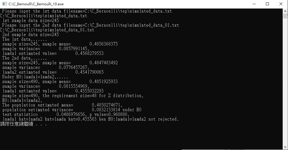
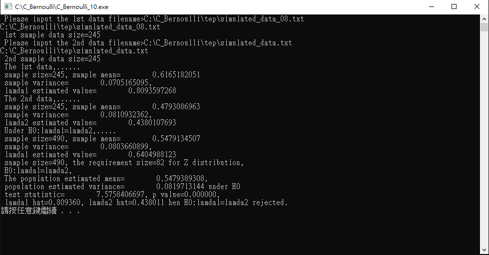
I simulate data named simulated_data.txt and simulated_data_01.txt from $CB(\lambda=0.4)$, simulated_data_08.txt from $CB(\lambda=0.8)$.
Figure 1 shows the test of two samples compared simulated_data.txt and simulated_data_01.txt. The $P value = 0.960880 > 0.05$ means that $H_{0}$ is not significantly rejected. The two data are significantly not different.
Test simulated_data_08.txt and simulated_data.txt. $P value = 0.000000 < 0.05$ means $H_{0}$ is significantly rejected. In fact, the two data are from different parameters of continuous Bernoulli distribution.
If your data were from continuous Bernoulli distribution, you can test two data if they have the same $\lambda$ value.